#30DayMapChallenge - Hexagons Map
Hexagons Theme for #30DayMapChallenge 2025. This interactive webmap is a bivariate analysis of Chicago taxi cab pick-up's and drop-off's in 2024 and 2025, using Uber's H3 hexagon grid as spatial units.
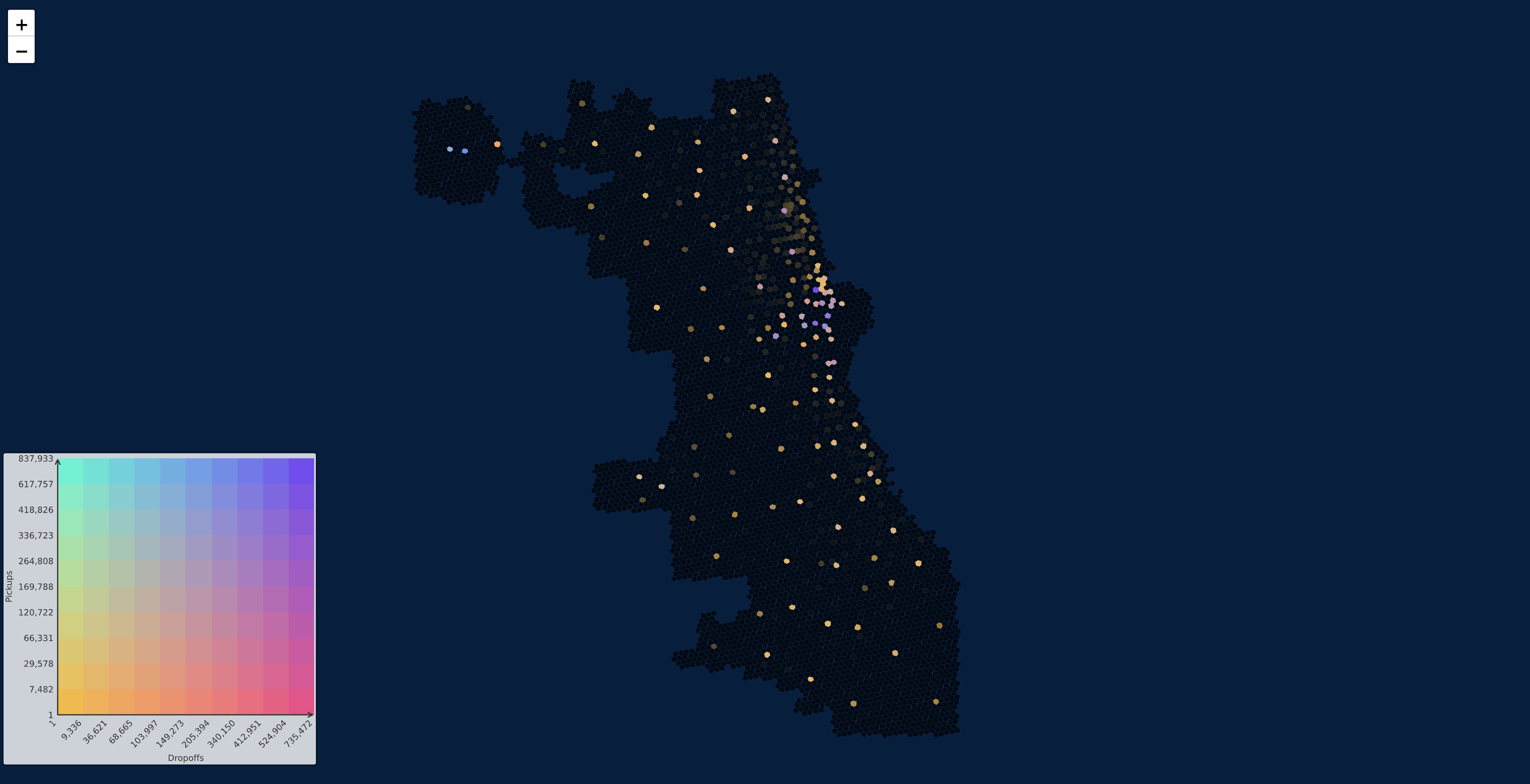
Bivariate Map of Taxi Cab Pick Up + Drop Off Locations in Chicago, 2024 - 2025
Bivariate Map of Taxi Cab Pick Up + Drop Off Locations in Chicago, 2024 - 2025
Click markers or scroll to explore
Bivariate Maps Illustate 2 Dimensions in a Choropleth Map
This gives us an understanding of place based on a range of outcomes balanced between 4 extremes. In this case, it illucidates which locations in Chicago might be pick up OR drop off hotspots, or BOTH.
The Coloring of Spatial Units Makes Patterns Clear
It's evident from the generally orange coloring across most of Chicago that outlying neighborhoods tend to be drop-off hotspots, rather than popular places to be picked up or a balance. This makes sense since residential neighborhoods tend to follow less regular commuting patterns in the evenings, during which transit services are less reliable or those returning from work or leisure opt for easier transportation home.
Bivariate Analysis Makes Pattern Outliers More Visible
This is clear in The Loop, where purple hexagons stand out in the crowd. These represent areas with a high proportion of both pick-ups and drop-offs, which makes sense given that most morning taxi trips will likely end here and the Central Business District provides the most passengers for pick-up in the evenings.
Code
hexagons_clean.pyimport csv
import re
import json
import jinja2
import numpy as np
import pandas as pd
import geopandas as gpd
import osmnx as ox
import h3
import folium
from shapely.geometry import Point, Polygon
from branca.element import Template, MacroElement
from bivario import explore_bivariate_data
# --- Paths ---
DATA_PATH = '/Users/mauricefarber/Downloads/Taxi_Trips_(2024-)_20251126.csv'
SHP_PATH = '/Users/mauricefarber/Documents/Personal Projects/30-Day Map Challenge/Data/chi_taxi.shp'
OUTPUT_PATH = '/Users/mauricefarber/Documents/Personal Projects/30-Day Map Challenge/Images/chicago_taxi_bivariate_naked.html'
# --- Load & clean CSV ---
data = pd.read_csv(DATA_PATH, on_bad_lines='skip', quoting=csv.QUOTE_NONE)
data.columns = data.columns.str.strip('"')
for col in ['Pickup Centroid Latitude', 'Pickup Centroid Longitude',
'Dropoff Centroid Latitude', 'Dropoff Centroid Longitude']:
if col in data.columns:
data[col] = data[col].astype(str).str.strip('"')
taxi = data.copy()
# --- Coordinate cleaning ---
def extract_point_values(val):
if pd.isna(val) or 'POINT' not in str(val):
return []
return [float(m) for m in re.findall(r'-?\d+\.?\d*', str(val))]
def clean_coord_pair(lat_val, lon_val):
lat_has_point = not pd.isna(lat_val) and 'POINT' in str(lat_val)
lon_has_point = not pd.isna(lon_val) and 'POINT' in str(lon_val)
if lat_has_point or lon_has_point:
all_vals = extract_point_values(lat_val) + extract_point_values(lon_val)
unique_vals = list(dict.fromkeys(all_vals))
if len(unique_vals) < 2:
return None, None
lon, lat = unique_vals[0], unique_vals[1]
else:
lat = pd.to_numeric(lat_val, errors='coerce')
lon = pd.to_numeric(lon_val, errors='coerce')
if pd.isna(lat) or pd.isna(lon):
return None, None
if 41.0 <= lat <= 43.0:
return lon, lat
return lat, lon
for prefix, lat_col, lon_col, x_col, y_col in [
('Pickup', 'Pickup Centroid Latitude', 'Pickup Centroid Longitude', 'Pickup X', 'Pickup Y'),
('Dropoff', 'Dropoff Centroid Latitude', 'Dropoff Centroid Longitude', 'Dropoff X', 'Dropoff Y'),
]:
results = taxi.apply(lambda row: clean_coord_pair(row[lat_col], row[lon_col]), axis=1)
taxi[x_col] = [r[0] if r[0] is not None else np.nan for r in results]
taxi[y_col] = [r[1] if r[1] is not None else np.nan for r in results]
taxi = taxi.dropna(subset=['Pickup X', 'Pickup Y', 'Dropoff X', 'Dropoff Y'])
taxi['Pickup Point'] = taxi.apply(lambda row: Point(row['Pickup X'], row['Pickup Y']), axis=1)
taxi['Dropoff Point'] = taxi.apply(lambda row: Point(row['Dropoff X'], row['Dropoff Y']), axis=1)
# --- Parse timestamps ---
taxi = taxi.rename(columns={"Taxi ID": "Time"})
taxi['Time'] = pd.to_datetime(taxi['Time'].str.strip('"'), errors='coerce')
# --- Chicago boundary ---
bound = ox.geocode_to_gdf("Chicago, IL")
chicago_geom = bound.geometry.iloc[0]
# --- H3 hexagons at resolution 9 ---
resolution = 9
center_lat, center_lon = chicago_geom.centroid.y, chicago_geom.centroid.x
center_hex = h3.latlng_to_cell(center_lat, center_lon, resolution)
minx, miny, maxx, maxy = chicago_geom.bounds
k_distance = int(max(maxx - minx, maxy - miny) * 50 * (resolution - 5))
hexagon_set = h3.grid_disk(center_hex, k_distance)
filtered_hexagons = [
hid for hid in hexagon_set
if chicago_geom.intersects(Polygon([(lon, lat) for lat, lon in h3.cell_to_boundary(hid)]))
]
hexagons_small = gpd.GeoDataFrame({
'hex_id': filtered_hexagons,
'geometry': [Polygon([(lon, lat) for lat, lon in h3.cell_to_boundary(hid)]) for hid in filtered_hexagons]
}, crs='EPSG:4326')
# --- Spatial join & aggregate counts ---
pickup_gdf = gpd.GeoDataFrame(taxi, geometry=taxi['Pickup Point'], crs=4326)
dropoff_gdf = gpd.GeoDataFrame(taxi, geometry=taxi['Dropoff Point'], crs=4326)
counts_pu = gpd.sjoin(pickup_gdf, hexagons_small, predicate='intersects')['hex_id'].value_counts().reset_index()
counts_do = gpd.sjoin(dropoff_gdf, hexagons_small, predicate='intersects')['hex_id'].value_counts().reset_index()
hex_gdf = hexagons_small.merge(counts_pu, on='hex_id').merge(counts_do, on='hex_id')
hex_gdf.to_file(SHP_PATH, driver='ESRI Shapefile', index=False)
# --- Reload from checkpoint ---
hex_gdf = gpd.read_file(SHP_PATH)
# --- Patch Jinja2 for bivario compatibility ---
_orig_env_init = jinja2.Environment.__init__
def _patched_env_init(self, *args, **kwargs):
_orig_env_init(self, *args, **kwargs)
self.filters['tojavascript'] = json.dumps
jinja2.Environment.__init__ = _patched_env_init
# --- Build bivariate map ---
m = folium.Map(location=[41.8781, -87.6298], zoom_start=10, tiles=None)
dark_bg = MacroElement()
dark_bg._template = Template("""
{% macro html(this, kwargs) %}
<style>
.leaflet-container { background: #001f3f !important; }
</style>
{% endmacro %}
""")
m.get_root().add_child(dark_bg)
folium.GeoJson(
hexagons_small,
style_function=lambda x: {
'fillColor': 'black',
'color': '#01376d',
'weight': 0.3,
'fillOpacity': 0.7,
},
name='Background Hexagons'
).add_to(m)
m = explore_bivariate_data(
hex_gdf,
"count_x",
"count_y",
column_a_label="Pickups",
column_b_label="Dropoffs",
scheme="natural_breaks",
k=10,
dark_mode=False,
cmap='kaleidoscope',
legend=True,
legend_size_px=300,
legend_background=True,
m=m,
)
m.save(OUTPUT_PATH)
print(f"Map saved to {OUTPUT_PATH}")Conclusion
Bivariate maps are a fantastic way to demonstrate the range of outcomes across two possible dimensions. The coloration makes outliers obvious and elucidate the spatial interaction between the two variables, which can be especially revealing with two very different measures. Moreover, Uber's increasingly popular H3 Hexagon grid, which minimizes error when quantifying movement through space at a very large scale, makes bivariate analysis look even better!