#30DayMapChallenge - Accessibility

April 25, 2026

Accessibility Theme for the #30DayMapChallenge 2025. Analyzing how accessible pubs are in London from each other using degree centrality and K-nearest neighbors in the city2graph Python package and discovering hidden clusters for a pub crawl.

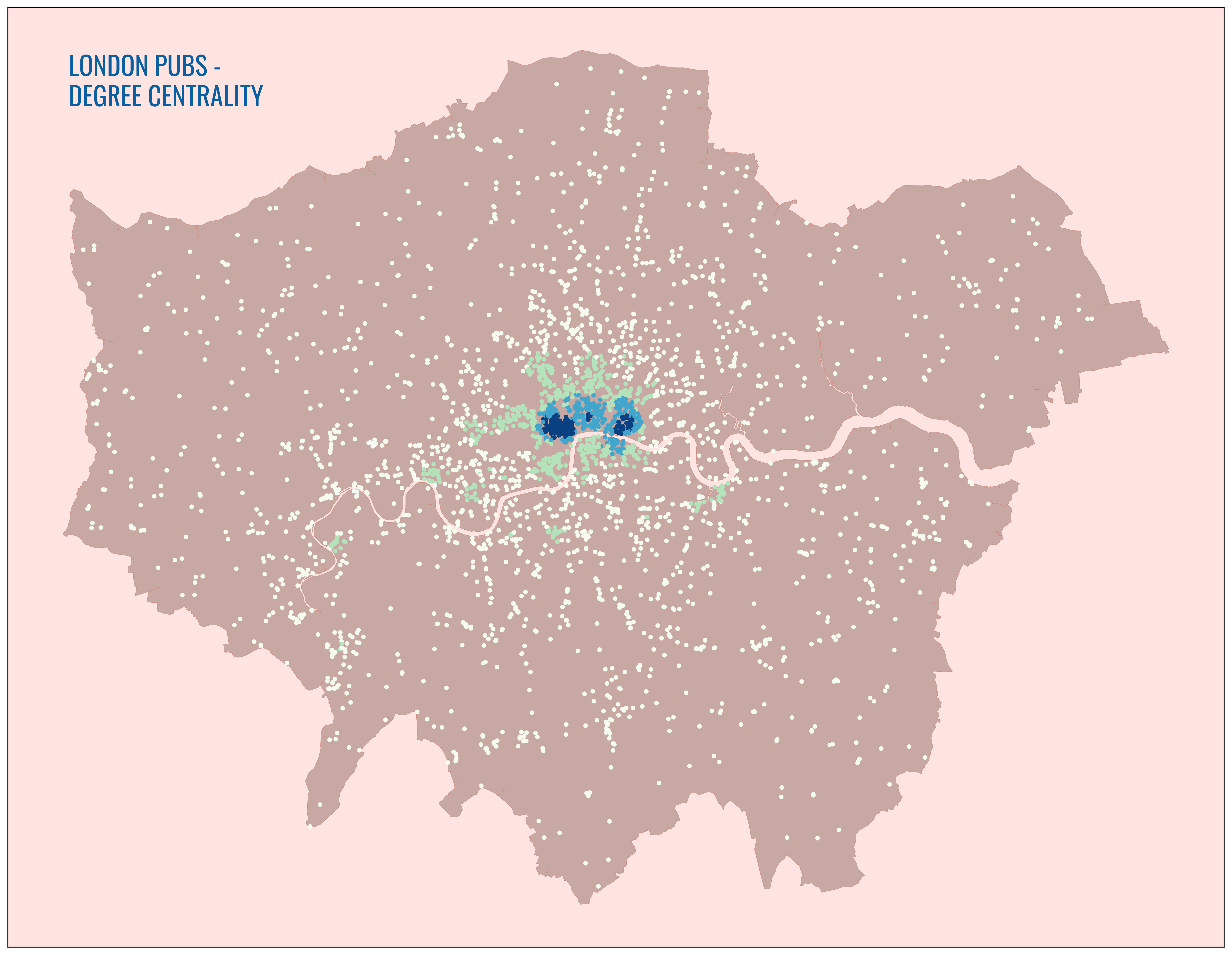
London Pubs - Degree Centrality

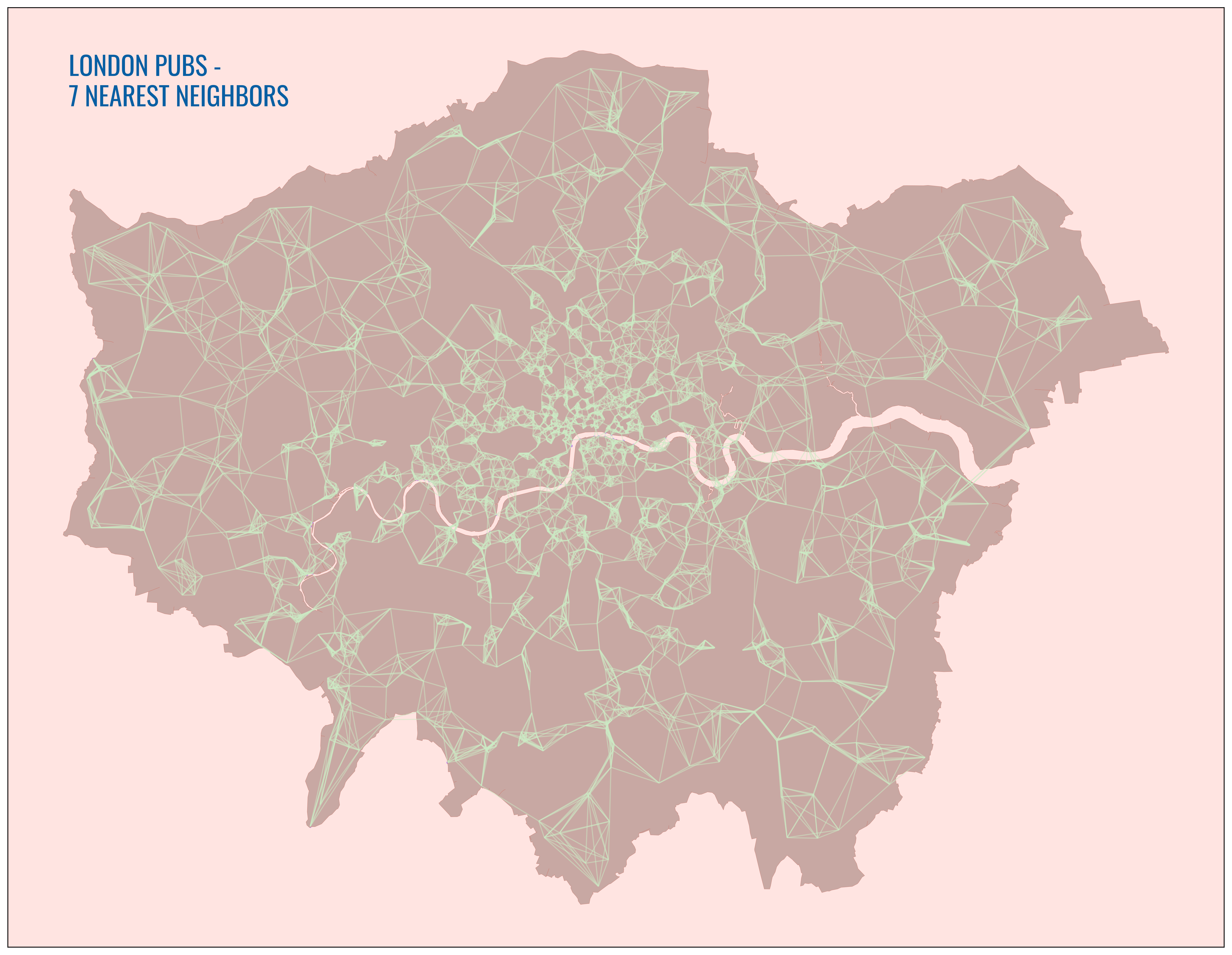
London Pubs - 7 Nearest Neighbors

London Pubs - Degree Centrality

Click markers or scroll to explore

Degree Centrality Measures Node Connectivity in a Network.

It quantifies the number of connections a node has to other similar nodes in a limited network. In this case, pubs are nodes and the limited network is all pubs within a 750 meter radius of any given pub.

Central London Pubs Have the Highest Degree Centrality

Intuitively, since Central London neighborhoods are the densest and have the most pubs, these pubs have the highest degree centrality. Within a short walk, you can reach more pubs from each pub in areas like Westminster and the City of London, therefore these pubs are considered more central to their limited networks, hence the shading.

London Pubs - 7 Nearest Neighbors

Click markers or scroll to explore

K-Nearest Neighbors Shows the Compactness of Like-Networks.

On a map, KNN shows where K other similar features in a set are to a principal feature, as far as the crow flies. In this case, it shows the 7 closest pubs to each pub in London. We can use this to find localized pub density across London.

Central London Has Many Small Networks of Pubs

This makes sense, since Central London neighborhoods have the highest density of pubs, therefore it takes far less distance to create completed networks of the 7 nearest pubs. For a group looking to do a pub-crawl, Central London is naturally the most logical location.

KNN Can Be Used to Discover Other Areas of High Localized Density

For instance, there is clearly there are relatively tightly-concentrated networks pubs in Greenwhich and Deptford. A group could recognize this as a fruitful spot for a pub crawl away from the Center.

KNN Elucidates Chains of Compact Networks

KNN is particularly useful outside of the more obvious urban core, providing further granularity than the Degree Centrality map. It makes evident chains of feature networks, useful for a group planning a long in multiple hotspotus outside of Central London.

Code

Day7_clean.py

python

import warnings
import numpy as np
import pandas as pd
import geopandas as gpd
import osmnx as ox
import networkx as nx
import matplotlib.pyplot as plt
import matplotlib.font_manager as fm
import contextily as ctx
import city2graph
from shapely.geometry import Point, LineString
from shapely.ops import polygonize

warnings.filterwarnings("ignore")

# --- Paths ---
PUBS_SHP    = '/Users/mauricefarber/Documents/Personal Projects/30-Day Map Challenge/Data/pubs.shp'
LONDON_SHP  = '/Users/mauricefarber/Documents/Personal Projects/Shapes/Greater London Boundary/Greater_London_Area_Boundary.shp'
FONT_PATH   = '/Users/mauricefarber/Downloads/Oswald/Oswald-VariableFont_wght.ttf'
OUT_KNN     = '/Users/mauricefarber/Documents/Personal Projects/30-Day Map Challenge/Images/london_pubs_knn.png'
OUT_CENT    = '/Users/mauricefarber/Documents/Personal Projects/30-Day Map Challenge/Images/london_pubs_deg_cent.png'

# --- Fetch pubs from OSM & save checkpoint ---
pubs = ox.features_from_place("Greater London", tags={"amenity": "pub"})

polys  = pubs[pubs.geometry.geom_type.isin(["Polygon", "MultiPolygon"])].copy()
polys.geometry = polys.geometry.centroid
points = pubs[pubs.geometry.geom_type == "Point"]
pubs   = pd.concat([points, polys])

pubs.to_file(PUBS_SHP, driver="ESRI Shapefile", index=False)

# --- Prepare POI GeoDataFrame (EPSG:27700) ---
poi_gdf = pubs.copy().reset_index()
poi_gdf["element"] = poi_gdf["element"].replace("way", "node")
poi_gdf = poi_gdf.set_index(["element", "id"]).to_crs(epsg=27700)

# --- London boundary → filled polygon ---
london = gpd.read_file(LONDON_SHP).to_crs(poi_gdf.crs)
filled_london = gpd.GeoSeries(list(polygonize(london.unary_union)), crs=london.crs)

# --- Street network (15 km radius from central London) ---
segments_G   = ox.graph_from_point((51.513361, -0.117464), dist=15000)
segments_gdf = ox.graph_to_gdfs(segments_G, nodes=False, edges=True)

# --- Helper: nx graph → node/edge GeoDataFrames ---
def graph_to_gdfs(graph, node_positions, crs=None):
    nodes = [
        {"node": n, "geometry": Point(x, y), "degree_centrality": graph.degree[n]}
        for n, (x, y) in node_positions.items()
    ]
    edges = [
        {"u": u, "v": v, "geometry": LineString([node_positions[u], node_positions[v]])}
        for u, v in graph.edges()
        if u in node_positions and v in node_positions
    ]
    return gpd.GeoDataFrame(nodes, crs=crs), gpd.GeoDataFrame(edges, crs=crs)

# --- Extract node positions ---
node_positions = {
    idx: (geom.x, geom.y) if geom.geom_type == "Point" else (geom.centroid.x, geom.centroid.y)
    for idx, geom in poi_gdf["geometry"].items()
}

# --- KNN graph (euclidean, k=7) for the network map ---
knn_net_nodes, knn_net_edges = city2graph.knn_graph(
    poi_gdf,
    distance_metric="euclidean",
    k=7,
    network_gdf=segments_gdf.to_crs(epsg=27700),
)

# --- Fixed-radius graph (750 m, euclidean) for degree centrality map ---
gil_l2_G = city2graph.fixed_radius_graph(
    poi_gdf,
    distance_metric="euclidean",
    radius=750,
    as_nx=True,
)
nodes_gdf, edges_gdf = graph_to_gdfs(gil_l2_G, node_positions, crs=poi_gdf.crs)

# --- Colors & font ---
_cmap       = plt.get_cmap("GnBu")
bg_color    = tuple(map(float, _cmap(0.25)))
title_color = tuple(map(float, _cmap(0.90)))

fm.fontManager.addfont(FONT_PATH)
plt.rcParams["font.family"] = "Oswald"

# --- Map 1: KNN network ---
fig, ax = plt.subplots(figsize=(20, 20))
knn_net_edges.plot(ax=ax, color=bg_color, alpha=0.5, linewidth=1)
knn_net_nodes.plot(ax=ax, color="#BF88EC", markersize=2)
filled_london.plot(ax=ax, color="#C8A8A3", linewidth=0.25, edgecolor="#CB847A")
ax.set_facecolor("mistyrose")
ax.set_xticks([]); ax.set_yticks([])
ax.set_xlabel(""); ax.set_ylabel("")
ax.text(0.05, 0.95, "LONDON PUBS - \n7 NEAREST NEIGHBORS",
        transform=ax.transAxes, fontsize=24, fontweight="bold",
        verticalalignment="top", color=title_color)
plt.savefig(OUT_KNN, dpi=400, bbox_inches="tight")
plt.close()

# --- Map 2: Degree centrality ---
fig, ax = plt.subplots(figsize=(20, 20))
filled_london.plot(ax=ax, color="#C8A8A3", linewidth=0.25, edgecolor="#CB847A")
nodes_gdf.plot(ax=ax, alpha=1, cmap="GnBu", column="degree_centrality",
               markersize=10, scheme="natural_breaks", k=4)
ax.set_facecolor("mistyrose")
ax.set_xticks([]); ax.set_yticks([])
ax.set_xlabel(""); ax.set_ylabel("")
ax.text(0.05, 0.95, "LONDON PUBS - \nDEGREE CENTRALITY",
        transform=ax.transAxes, fontsize=24, fontweight="bold",
        verticalalignment="top", color=title_color, fontname="Oswald")
plt.savefig(OUT_CENT, dpi=400, bbox_inches="tight")
plt.close()

Conclusion

Both Degree Centrality and K-Nearest Neighbors analyses are great for assessing accessibility of a feature in regards to its relations to similar features. In practical terms, it allows for more efficient route and location planning and is applicable across use cases, whether location planning for a logistics center or planning a pub crawl with mates. Both tools work together to reveal different levels of granularity and both layers work in concert to qualify accessibility in a metropolitan area.